Uncertainty Quantification

MADS is applied to perform uncertainty quantification using Bayesian sampling.

The analyses below are performed using examples/bayesian_sampling/bayesian_sampling.jl.

Model setup

There are:

• Contaminant source (yellow rectangle)
• 3 monitoring wells (W1, W2, and W3; blue dots)

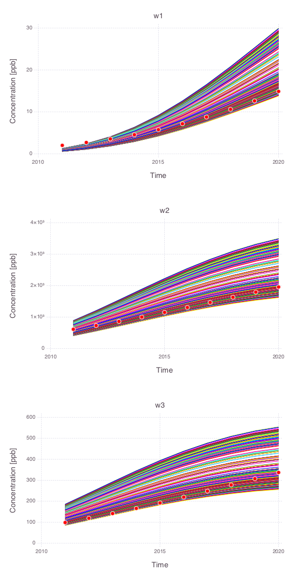
Prior spaghetti plots

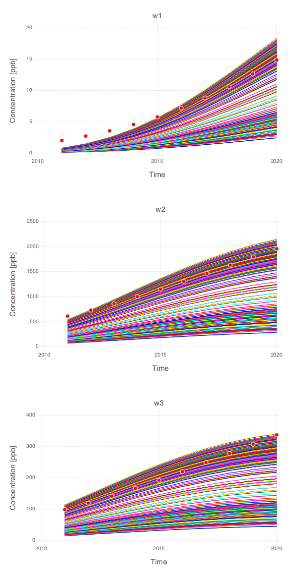
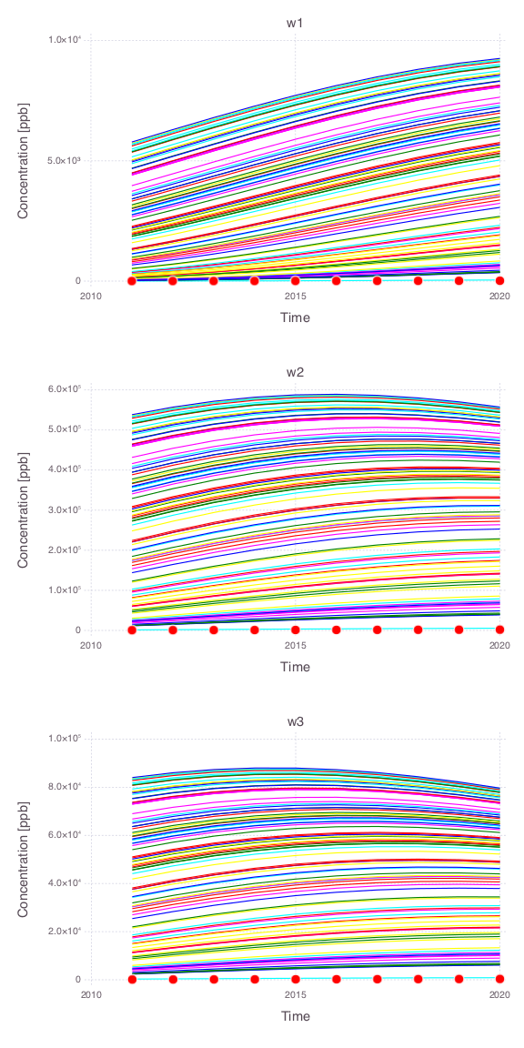
Below we show joint and individual spaghetti plots of 100 model runs representing the prior model prediction uncertainties at the 3 monitoring wells.

Joint spaghetti plots

All model parameters are changed simultaneously within their prior uncertainty ranges.

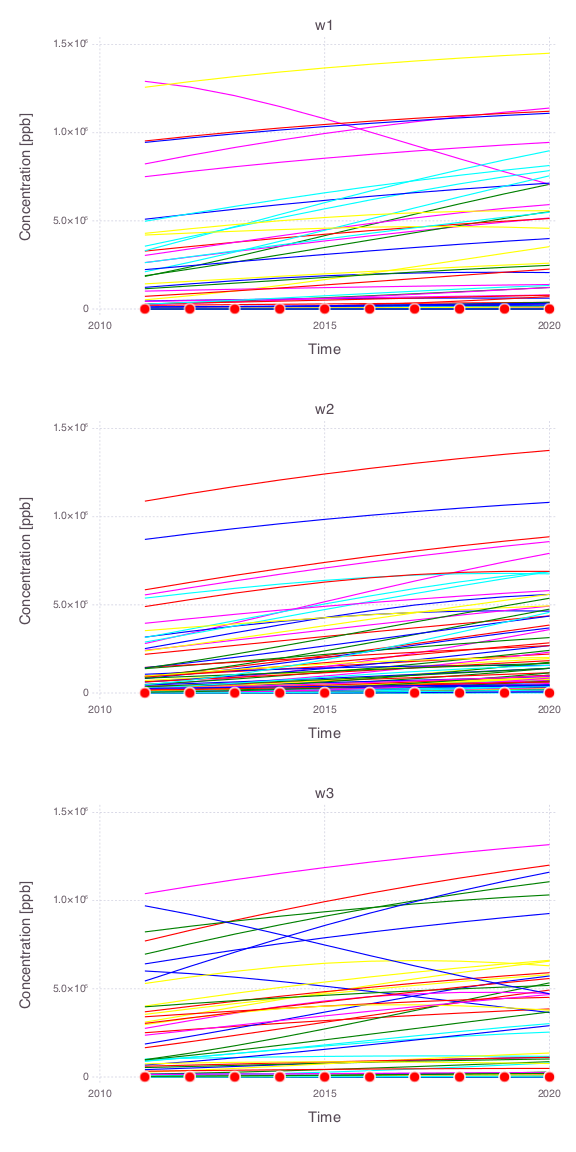
Individual spaghetti plots

A single model parameter is changed at a time.

• Source $x$ location

• Source $y$ location

• Source size along $x$ axis

• Source size along $y$ axis

• Source release time $t_0$

• Source termination time $t_1$

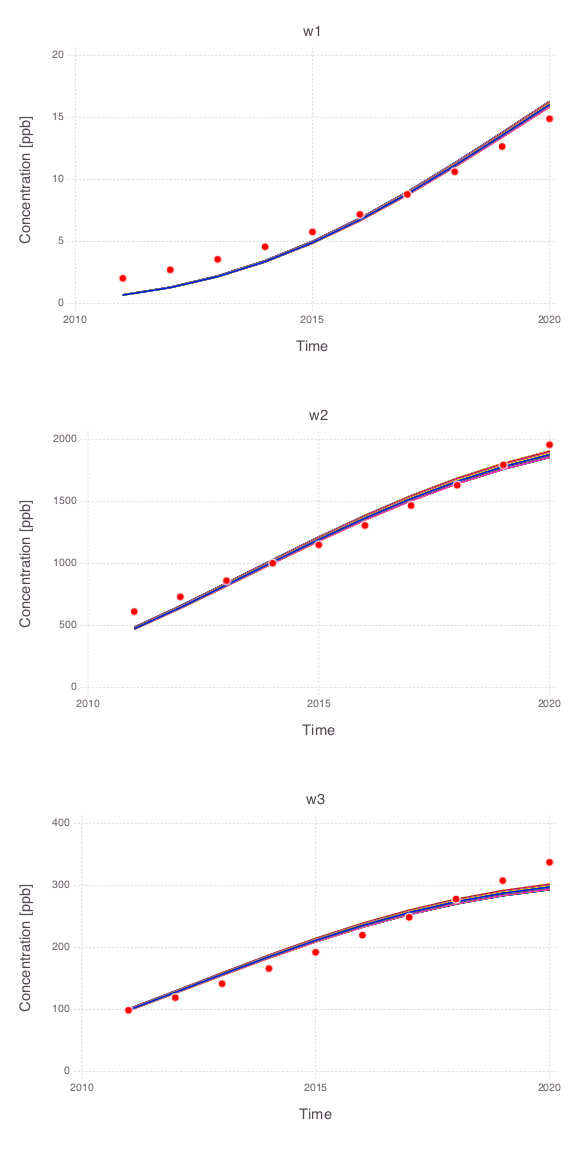
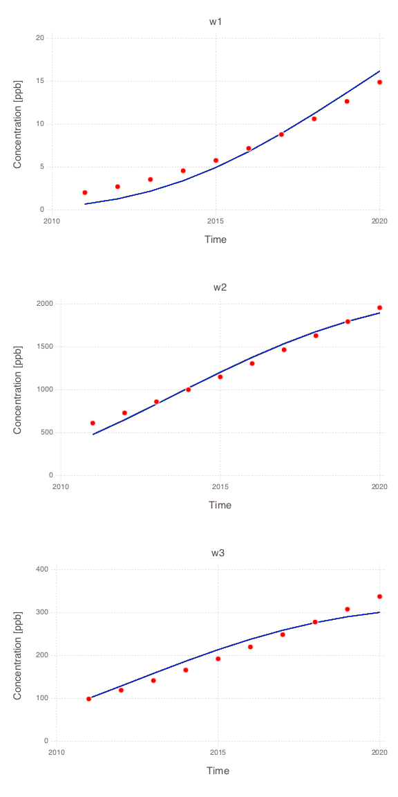
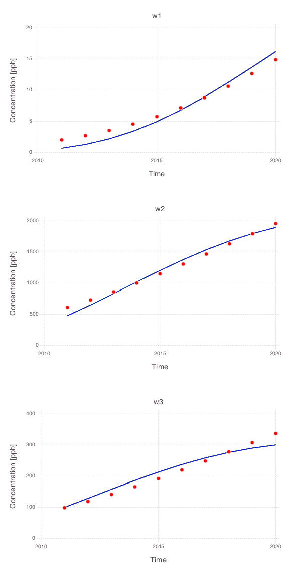
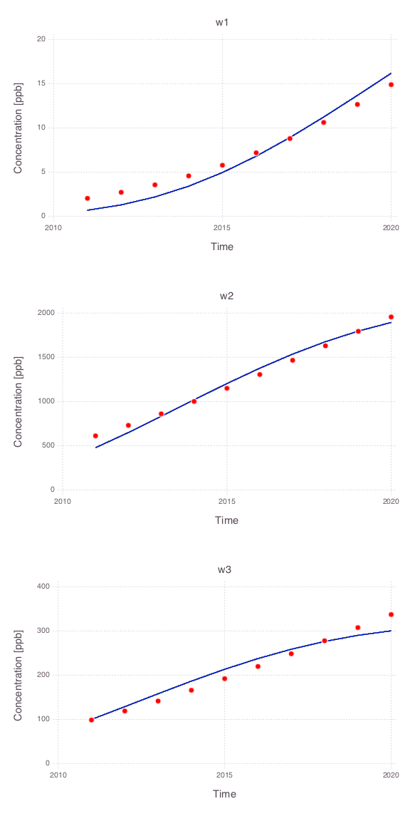
Model calibration match

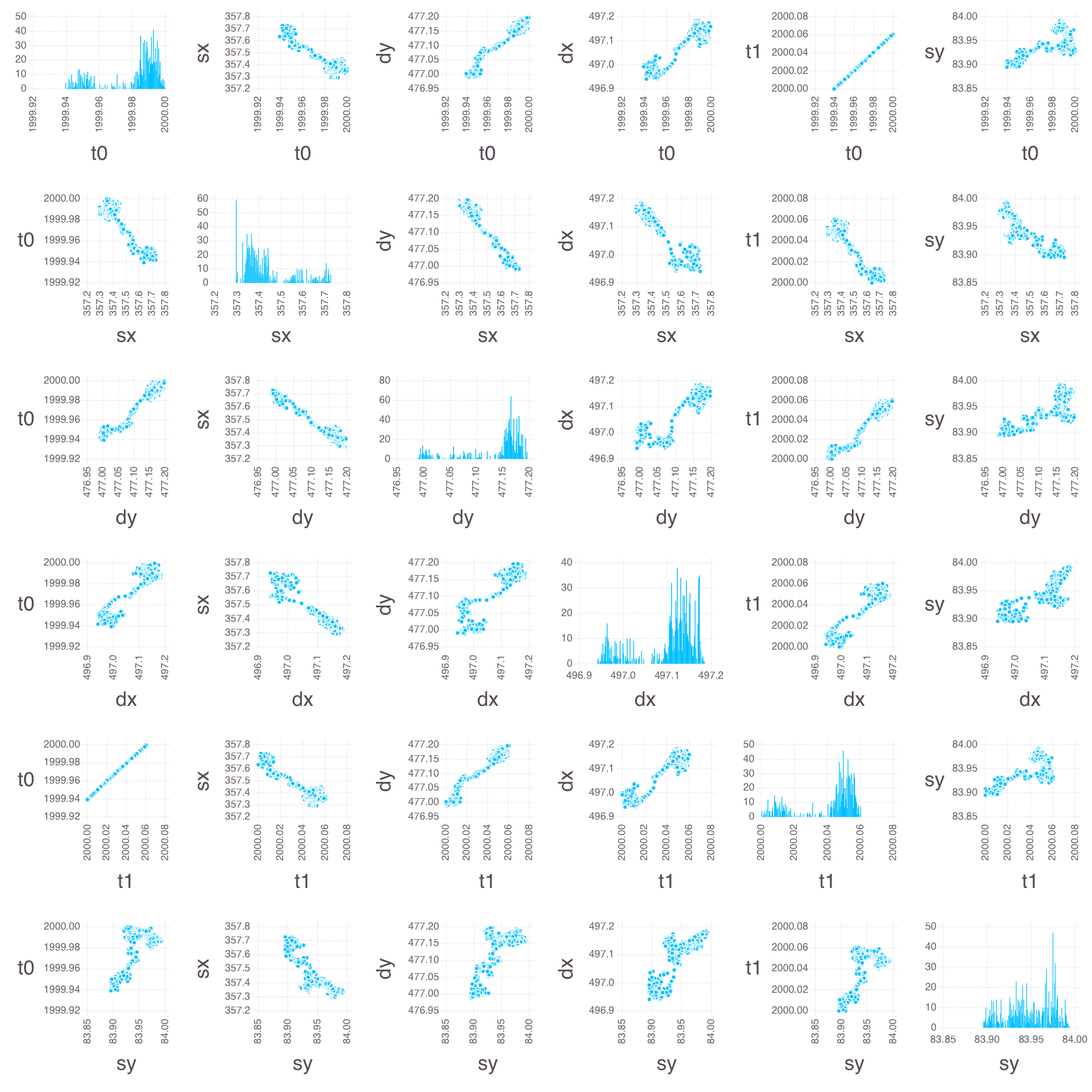
Bayesian sampling results

Posterior spaghetti plots

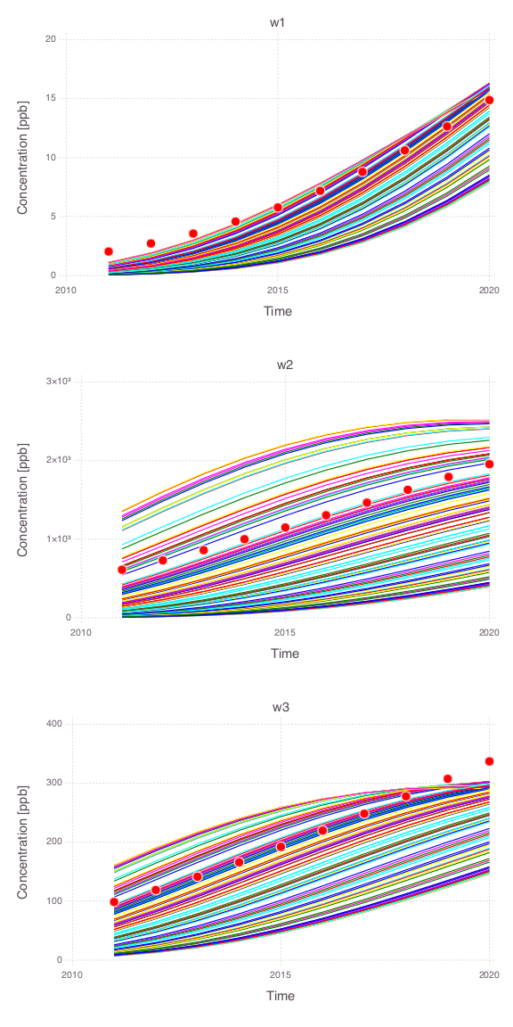
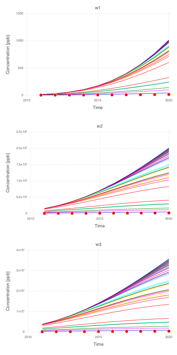
Spaghetti plots of 1000 model predictions representing the posterior model uncertainties at the 3 monitoring wells.

Joint spaghetti plots

All model parameters are changed simultaneously within their prior uncertainty ranges.

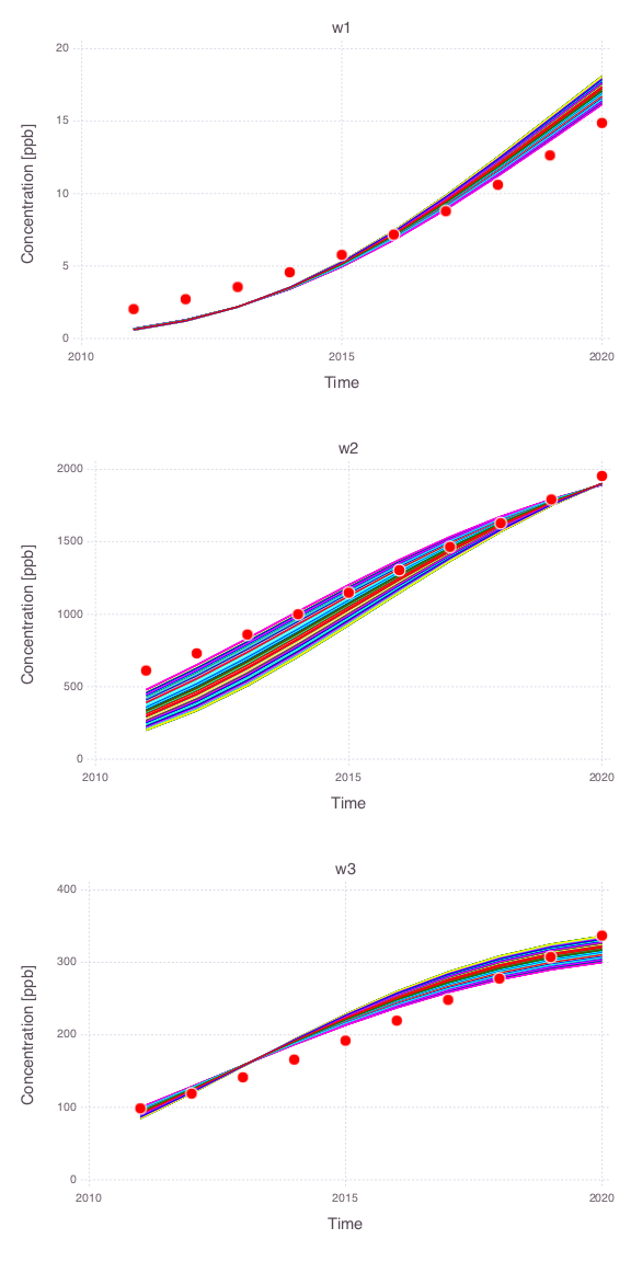
Individual spaghetti plots

A single model parameter is changed at a time.

Note that only the posterior uncertainties in the source release time ($t_0$) and the source termination time ($t_1$) are producing large impact in the model predictions.

• Source $x$ location (all the 1000 model predictions are overlapping)

• Source $y$ location (all the 1000 model predictions are overlapping)

• Source size along $x$ axis (all the 1000 model predictions are overlapping)

• Source size along $y$ axis (all the 1000 model predictions are overlapping)

• Source release time $t_0$

• Source termination time $t_1$