Model Calibration for Contamination Problem

MADS is applied to solve a general groundwater contamination problem using model inversion.

MADS includes an analytical solver called Anasol.jl to solve the groundwater contamination transport in an aquifer.

Problem setup

import Mads

Setup the working directory

cd(joinpath(Mads.dir, "examples", "contamination"))

Load MADS input file

md = Mads.loadmadsfile("w01.mads")

Dict{String, Any} with 7 entries:
  "Grid"         => Dict{Any, Any}("zmax"=>50, "time"=>50, "xcount"=>33, "zcoun…
  "Sources"      => Dict{Any, Any}[Dict("box"=>Dict{Any, Any}("dz"=>Dict{Any, A…
  "Parameters"   => OrderedCollections.OrderedDict{String, OrderedCollections.O…
  "Wells"        => OrderedCollections.OrderedDict{String, Any}("w1a"=>Dict{Any…
  "Time"         => Dict{Any, Any}("step"=>1, "start"=>1, "end"=>50)
  "Observations" => OrderedCollections.OrderedDict{Any, Any}("w1a_1"=>OrderedCo…
  "Filename"     => "w01.mads"

Plot

Generate a plot of the loaded problem showing the well locations and the location of the contaminant source:

Mads.plotmadsproblem(md, keyword="all_wells")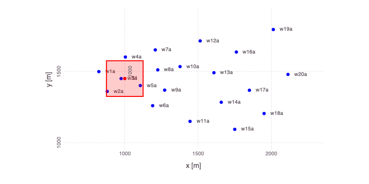

There are 20 monitoring wells.

Each well has 2 measurement ports:

• shallow (3 m below the water table labeled a) and
• deep (33 m below the water table labeled b).

Contaminant concentrations are observed for 50 years at each well.

The contaminant transport is solved using the Anasol package in MADS.

Unknown model parameters

• Start time of contaminant release (t_0)
• End time of contaminant release (t_1)
• Advective pore velocity (v)

Reduced model setup

Analysis of the data from only 2 monitoring locations: w13a and w20a.

Mads.allwellsoff!(md) # turn off all wells
Mads.wellon!(md, "w13a") # use well w13a
Mads.wellon!(md, "w20a") # use well w20a

OrderedCollections.OrderedDict{Any, Any} with 100 entries:
  "w13a_1"  => OrderedCollections.OrderedDict{Any, Any}("well"=>"w13a", "time"=…
  "w13a_2"  => OrderedCollections.OrderedDict{Any, Any}("well"=>"w13a", "time"=…
  "w13a_3"  => OrderedCollections.OrderedDict{Any, Any}("well"=>"w13a", "time"=…
  "w13a_4"  => OrderedCollections.OrderedDict{Any, Any}("well"=>"w13a", "time"=…
  "w13a_5"  => OrderedCollections.OrderedDict{Any, Any}("well"=>"w13a", "time"=…
  "w13a_6"  => OrderedCollections.OrderedDict{Any, Any}("well"=>"w13a", "time"=…
  "w13a_7"  => OrderedCollections.OrderedDict{Any, Any}("well"=>"w13a", "time"=…
  "w13a_8"  => OrderedCollections.OrderedDict{Any, Any}("well"=>"w13a", "time"=…
  "w13a_9"  => OrderedCollections.OrderedDict{Any, Any}("well"=>"w13a", "time"=…
  "w13a_10" => OrderedCollections.OrderedDict{Any, Any}("well"=>"w13a", "time"=…
  "w13a_11" => OrderedCollections.OrderedDict{Any, Any}("well"=>"w13a", "time"=…
  "w13a_12" => OrderedCollections.OrderedDict{Any, Any}("well"=>"w13a", "time"=…
  "w13a_13" => OrderedCollections.OrderedDict{Any, Any}("well"=>"w13a", "time"=…
  "w13a_14" => OrderedCollections.OrderedDict{Any, Any}("well"=>"w13a", "time"=…
  "w13a_15" => OrderedCollections.OrderedDict{Any, Any}("well"=>"w13a", "time"=…
  "w13a_16" => OrderedCollections.OrderedDict{Any, Any}("well"=>"w13a", "time"=…
  "w13a_17" => OrderedCollections.OrderedDict{Any, Any}("well"=>"w13a", "time"=…
  "w13a_18" => OrderedCollections.OrderedDict{Any, Any}("well"=>"w13a", "time"=…
  "w13a_19" => OrderedCollections.OrderedDict{Any, Any}("well"=>"w13a", "time"=…
  "w13a_20" => OrderedCollections.OrderedDict{Any, Any}("well"=>"w13a", "time"=…
  "w13a_21" => OrderedCollections.OrderedDict{Any, Any}("well"=>"w13a", "time"=…
  "w13a_22" => OrderedCollections.OrderedDict{Any, Any}("well"=>"w13a", "time"=…
  "w13a_23" => OrderedCollections.OrderedDict{Any, Any}("well"=>"w13a", "time"=…
  "w13a_24" => OrderedCollections.OrderedDict{Any, Any}("well"=>"w13a", "time"=…
  "w13a_25" => OrderedCollections.OrderedDict{Any, Any}("well"=>"w13a", "time"=…
  â‹®         => â‹®

Generate a plot of the updated problem showing the 2 well locations applied in the analyses as well as the location of the contaminant source:

Mads.plotmadsproblem(md; keyword="w13a_w20a")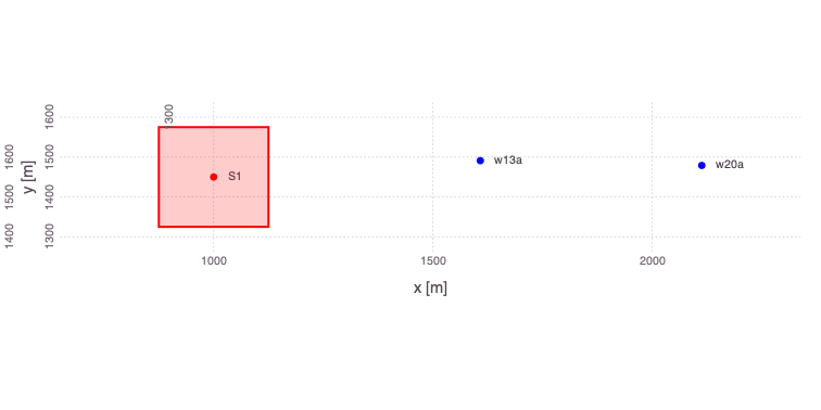

Initial estimates

Plot initial estimates of the contamiant concentrations at the 2 monitoring wells based on the initial model parameters:

• w13a

Mads.plotmatches(md, "w13a"; display=true)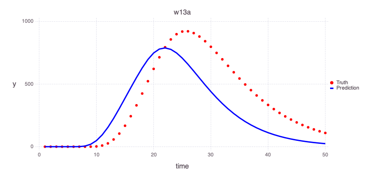

• w20a

Mads.plotmatches(md, "w20a"; display=true)

Model calibration

Execute model calibration based on the concentrations observed in the two monitoring wells:

calib_param, calib_results = Mads.calibrate(md)

Compute forward model predictions based on the calibrated model parameters:

calib_predictions = Mads.forward(md, calib_param)

OrderedCollections.OrderedDict{Any, Float64} with 100 entries:
  "w13a_1"  => 0.0
  "w13a_2"  => 0.0
  "w13a_3"  => 0.0
  "w13a_4"  => 0.0
  "w13a_5"  => 0.0
  "w13a_6"  => 4.79956e-11
  "w13a_7"  => 0.000284228
  "w13a_8"  => 0.0590933
  "w13a_9"  => 0.92868
  "w13a_10" => 5.08796
  "w13a_11" => 16.2469
  "w13a_12" => 37.7882
  "w13a_13" => 71.6886
  "w13a_14" => 118.275
  "w13a_15" => 176.509
  "w13a_16" => 244.465
  "w13a_17" => 319.785
  "w13a_18" => 400.036
  "w13a_19" => 482.934
  "w13a_20" => 566.28
  "w13a_21" => 647.03
  "w13a_22" => 720.732
  "w13a_23" => 782.658
  "w13a_24" => 829.249
  "w13a_25" => 858.781
  â‹®         => â‹®

Plot the predicted estimates of the contamiant concentrations at the 2 monitoring wells based on the estimated model parameters based on the performed model calibration:

• w13a

Mads.plotmatches(md, calib_predictions, "w13a")

• w20a

Mads.plotmatches(md, calib_predictions, "w20a")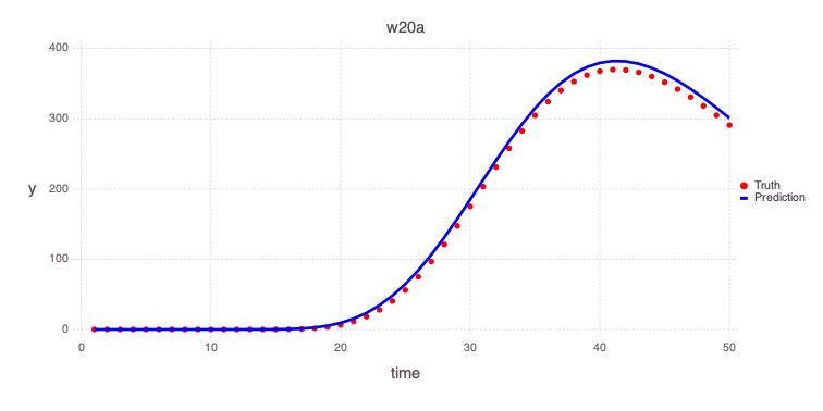

Initial values of the optimized model parameters are:

Mads.showparameters(md)

Pore x velocity [L/T] : vx       =              40 log-transformed min = 0.01 max = 200.0
Start Time [T]        : source1_t0 =               4 min = 0.0 max = 10.0
End Time [T]          : source1_t1 =              15 min = 5.0 max = 40.0
Number of optimizable parameters: 3

Estimated values of the optimized model parameters are:

Mads.showparameterestimates(md, calib_param)

3-element Vector{Pair{String, Float64}}:
         "vx" => 31.059669248076222
 "source1_t0" => 5.036614115598699
 "source1_t1" => 16.62089724181972